Every week Digital Humanities Now (DHNow) distributes the most important news and pieces for the field by publishing links on our website and Twitter feed. In order to identify the content most valuable to this broad and dispersed community, we rely on volunteers who help us read through the aggregated RSS feeds from our collection of 500+ identified sources, as well as content identified by searches on the open web.
It is not easy to review approximately 1,000 items a week in order to find the 3-4 DHNow “Editors’ Choice” pieces that move the field forward, and the 15-20 news items of greatest importance. Most of the items that flow into our RSS pool do not fit into the category of news or scholarly communication about the practice of digital humanities. It takes time and energy to wade through this large pool of documents, and we have often longed for a filter for this river of news that would surface the most promising pieces for careful consideration. Right now we have volunteer editors acting as a filter. But we also wanted to explore the potential for automatic identification of content, based on a customized set of priorities.
With this goal in mind, we began working with Xin Guan, a graduate student of computer science at George Mason University, who is studying machine learning. Guan’s experiment was to develop a classifier program that would use data mining methods in order to identify potentially valuable content. To help with the identification, we gave him all the items in the river of news from the month of July 2012 (approximately 2,500 documents) as well as the 235 Editors’ Choice selections from 11 months of publishing.
We hoped that he could train a classifier program to value the qualities of the “accepted” class of documents (the Editors’ Choice pieces) with enough precision to identify other documents in the pool that had similar qualities, and “reject” the rest.
Our experiment ends well. We reviewed the content identified by the classifier several times, in order to help refine the method. In December 2012 the classifier program sifted through a new pool of items from the river of news and identified 40 “accepted” documents. Indeed, all 40 “accepted” items were either published, or worthy of publishing, in DHNow.
With a little more work on the interface and method, we anticipate incorporating the classifier program into our weekly workflow. After this next round of experimentation, we plan to share results, as well as the program itself, with everyone.
Those interested in the concepts and logistics behind the classifier program will be interested to read the rest of this post, in which Xin Guan explains how he used the Active Learning method of Machine Learning in order to train the classifier program.
Applying Active Learning SVM to Scholarly Writing from the Open Web
Active Learning Classification Framework
For the purposes of this experiment, the Editors of DHNow provided a large pool of approximately 2,500 documents. The documents could be labeled with only one possible class, out of two options: “accept” or “reject.” Also delivered were 235 “accepted” documents that had been published as Editors’ Choice pieces over the course of 11 months. The goal was to identify documents in the larger pool that had qualities similar to those provided as examples of “accepted” documents. And if it works fine on the pool, we could expect it will have a good performance on the future documents.
We consider this problem as a binary classification problem, and build a classifier to deal with it, named Active Learning Support Vector Machine (SVM). In our problem, a classifier means a Machine Learning model that decides which class a document belongs to. Active Learning is the framework, and SVM is the classifier software program based on Java. And now, let’s see what they mean.
Before introducing Active Learning SVM, I need to introduce some technical terminology.
- “instance” — In our problem, an “instance” is a document. And in order to make sure that a computer can understand the document, we use the number of occurrences of a word in a document to represent it. This information is stored in a high-dimension vector: each dimension represents a specific word, and the value is the number of occurrences of that word, so each instance (document) is a vector.
- “label” — Every instance should have a label. A “ground truth label” means which class the instance really belongs to. A label obtained by classifier is the class the classifier thinks the instance should belong to. In our problem, label has two values, ‘Accept’ or ‘reject’.
- “training data set” — A set of instances with ground truth label, used to build our classifier.
- “testing data set” — Usually we will separate a subset from training data set as testing data set. The instances in testing data set will not be used during training process. The goal of the testing set is to evaluate the performance of the classifier. We will blind the ground truth label and get the label by classifier. And then compare the result with ground truth label to check the performance of the classifier on the future data.
And now let’s introduce Active Learning framework. The idea of Active Learning is that, unlike traditional classification framework, it evolves an oracle (such as a human) in the process, and builds a loop to iteratively improve the performance of the classifier. What does an oracle do? He gives the ground truth label to some of the instances in order to give more information to the classifier, and then the classifier will update itself with this information.
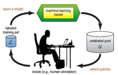
Figure 1 shows how Active Learning works. In our case, the process is as following.
- First, we use some known instances and labels to get a classifier (the machine learning model in Figure 1). The classifier will go through all the documents without knowing the labels, and find out the documents for which it is hard to decide whether to ‘accept’ or not.
- Then the oracle will read these documents and decide to accept or reject each of them (in this case acceptance would mean that is acceptable for publishing on DHNow)
- With all the information, the classifier will retrain and adjust itself to be more suitable to this problem. Another loop will start, until the user is satisfied with the performance.
Active learning is well-motivated in many modern machine learning problems where data may be abundant but labels are scarce or expensive to obtain. The goal is to reduce the need of the labels of instances as few as possible. It also has better performance when the data is imbalanced, because the classifier will automatically choose the most “valuable” instances from the unlabeled instances pool.
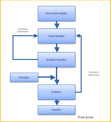
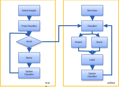
To show the differences between Active Learning classification and normal classification, see the flow charts in Figure 2 and Figure 3. From the flow chart and the above statements we see that the most important difference between the normal classifier and active learning classifier is how the training data was given. In normal classifiers, the training samples are usually given by random, while in active learning classifier, it will query several instances from a large unlabeled instances pool not based on random choice, but based on the query strategies. And these selected instances will be given the ground truth label and then join in the training data set for the classifier to update.
Details on the Classifier
To use the Active learning algorithm in this problem, we choose to implement SVM as the classifier (machine learning model). For updating the classifier after each query, we just re-train the SVM with the given instances with label and add the new queried instances. For the query strategy, we choose the instances that close to the hyper-plane and with high variance to the training data set. Figure 4 shows the support vectors and helps explain how the intuitive query works.
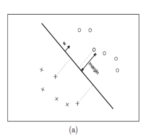
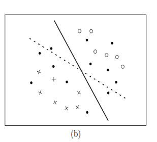
Now I will explain the query strategy in detail. As shown in Figure 4, every point in the figure represents one instance. The coordinate of the instance is based on the vector which we discussed previously. The distance between two points is the similarity of two documents in the feature space. The documents which are close to each other means the words they contain are similar, and the content of these documents can be considered related in some degree. The solid circles represent unlabeled instances. Each x or circle represents a labeled instance (‘accept’ or ‘reject’). The solid line is the current hyper-plane based on labeled instances, which helps the classifier decide the class label for documents. And the dot line is the ground truth hyper-plane we want to get. To query instances from unlabeled data, an intuitive way is to select the instances that are close to hyper-plane, because if these instances’ labels are known, the hyper-plane will have more constrains and be limited to a certain space, called version space. Simon Tong (2001) proved that selected these instances will quickly reduce the size of the version space, and then get the hyper-plane that very close to the truth.[2] The distance is calculated by formula (1). And we will query the instances which have the minimum value of distance.
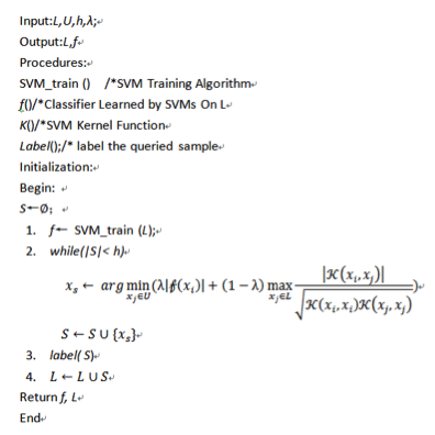
King-Shy Goh et al (2004) supposed that the queried instances should contain some information that the current labeled data set does not have. So they proposed a query method called angle diversity, which besides considering the distance to the hyper-plane, also considering the queried instances’ max cosine value to the already labeled instances. They assume such instances would be more helpful to the future data. They use formula 3 to get the score of unlabeled instances, and query the lowest one.[3]
Implementation
That’s all about the theory. Now we will implement it. First, pre-process the data set to vector. The data set are downloaded by Google reader API, and it is a XML file. After the common pre-process for documents, including change to lowercase letter, delete stop words, transform to the vector based on dictionary. Thanks to the Mallet project, we can easily do the above process using their open source library.[4] Second, SVM is a well-known classifier algorithm, and we use libSVM for Java in our project.[5] For Active Learning SVM implementation, according to the formula stated in previous part, we can have the pseudo- code for Active Learning SVM as follows:
Performance
How about the performance? We have 2736 instances in training data in total, in which 235 are ‘accept’, and rest of them are ’reject’. Based on our classifier’s result, we get around 95% of accuracy, 77% of recall, and 74% of precision. And when we try this on the new incoming data, it really works. As a test case we used new documents produced during the first two week of December 2012. There were 40 “accept” instances, and all 40 also were accepted by the editors. In many cases the posts had been selected for publication through the traditional process of editorial review. But the classifier also identified some valuable pieces which were missed by the editors — so they were selected for publishing the next day. This means that the classifier makes good recommendations and will help the editors a lot.
A more formal report about this project is available here.
References
- Burr Settles. 2009. “Active Learning Literature Survey.” Computer Sciences Technical Report 1648. University of Wisconsin–Madison.
- Simon Tong, Daphne Koller. 2001. “Support Vector Machine Active Learning with Application to Text Classification.” Journal of Machine Learning Research (2001): 45-66.
- King-Shy Goh, Edward Y. Chang, and Wei-Cheng Lai. 2004. “Multimodal concept-dependent active learning for image retrieval.” In Proceedings of the 12th annual ACM international conference on Multimedia(MULTIMEDIA ’04). ACM, New York, NY, 564-571.
- Andrew Kachites McCallum. 2002. “MALLET: A Machine Learning for Language Toolkit.” http://mallet.cs.umass.edu.
- Chih-Chung Chang and Chih-Jen Lin. 2011. “LIBSVM : a library for support vector machines.” ACM Transactions on Intelligent Systems and Technology: 2:27:1–27:27. Software available at http://www.csie.ntu.edu.tw/~cjlin/libsvm.
- Figure from King-Shy Goh, Edward Y. Chang, and Wei-Cheng Lai. 2004. “Multimodal concept-dependent active learning for image retrieval.” In Proceedings of the 12th annual ACM international conference on Multimedia (MULTIMEDIA ’04). ACM: 564-571.

